1. Re-center Particles

How to update particle location centers from alignments in 2D Classification data.

Before proceeding, install the cryosparc-tools module in your Python environment. Also ensure CryoSPARC base ports +2 and +3 (40002 and 40003 in this example) are available on this machine.

The following python dependencies are also required to render results and may be installed with conda or pip:

• pandas

• matplotlib

• numpy (included with cryosparc-tools)

First initialize the CryoSPARC client:

from cryosparc.tools import CryoSPARC

cs = CryoSPARC(host="cryoem5", base_port=40000)
assert cs.test_connection()

Connection succeeded to CryoSPARC command_core at http://cryoem5:40002
Connection succeeded to CryoSPARC command_vis at http://cryoem5:40003

This instance has a 2D Classification and Select 2D Classes job at P251-J15 and P251-J16, respectively. Re-extract those selected particles with updated centers computed by the 2D Classification job.

First retrieve the job handle and its particles output with the load_output method.

project = cs.find_project("P251")
job = cs.find_job("P251", "J16")
particles = job.load_output("particles_selected")

Get a subset of relevant columns and display the first 10 rows as a pandas dataframe:

import pandas as pd

first_10 = particles.slice(0, 10)
first_10 = first_10.filter_fields(
    [
        "alignments2D/psize_A",
        "alignments2D/shift",
        "blob/psize_A",
        "location/center_x_frac",
        "location/center_y_frac",
        "location/micrograph_shape",
    ]
)
pd.DataFrame(first_10.rows())

	alignments2D/psize_A	alignments2D/shift	blob/psize_A	location/center_x_frac	location/center_y_frac	location/micrograph_shape	uid
0	2.30125	[-5.2, -2.6]	0.6575	0.934483	0.753333	[7676, 7420]	12660056651751289214
1	2.30125	[-5.2, 7.8]	0.6575	0.627586	0.163333	[7676, 7420]	17971771557537199412
2	2.30125	[-5.2, 0.0]	0.6575	0.413793	0.448333	[7676, 7420]	17954957875627625872
3	2.30125	[-5.2, 7.8]	0.6575	0.441379	0.311667	[7676, 7420]	5996321661655483102
4	2.30125	[2.6, 10.4]	0.6575	0.603448	0.088333	[7676, 7420]	9631994642463500771
5	2.30125	[-13.0, 0.0]	0.6575	0.860345	0.720000	[7676, 7420]	16429739213182044957
6	2.30125	[0.0, 7.8]	0.6575	0.924138	0.563333	[7676, 7420]	15428131659279662499
7	2.30125	[-2.6, 0.0]	0.6575	0.925862	0.926667	[7676, 7420]	10124600487485993501
8	2.30125	[2.6, -5.2]	0.6575	0.482759	0.445000	[7676, 7420]	644635160388285141
9	2.30125	[2.6, 2.6]	0.6575	0.039655	0.228333	[7676, 7420]	2866600664684787659

Each particle has [location/center_x_frac, location/center_y_frac] fields which contain the fractional distance of each particle from the top-left corner of the micrograph. By convention, the top-left corner of the micrograph is [0, 0] and the bottom right corner is [1, 1].

Use the shifts calculated by the 2D Classification job to modify the particle location. These are located at alignments2D/shift for each particle. The shift units are in pixels with pixel size alignments2D/psize_A (used during original computation of the 2D Class Averages).

Convert the original locations to pixels before doing the shift operation for increased floating point precision.

class2d_psize = particles["alignments2D/psize_A"]
micrograph_psize = particles["blob/psize_A"]

mic_shape_y, mic_shape_x = particles["location/micrograph_shape"].T
shift_x = class2d_psize * particles["alignments2D/shift"][:, 0] / micrograph_psize
shift_y = class2d_psize * particles["alignments2D/shift"][:, 1] / micrograph_psize
new_loc_x = particles["location/center_x_frac"] * mic_shape_x - shift_x
new_loc_y = particles["location/center_y_frac"] * mic_shape_y - shift_y

Create a copy of the particles dataset where the results are be saved. Convert the new locations back to fractions and reset the shift.

updated_particles = particles.copy()
updated_particles["location/center_x_frac"] = new_loc_x / mic_shape_x
updated_particles["location/center_y_frac"] = new_loc_y / mic_shape_y
updated_particles["alignments2D/shift"][:] = [0, 0]

Next, plot these particles onto a sample micrograph to check that the new locations were calculated correctly. First download the micrograph for one of the particles.

mic_path = particles["location/micrograph_path"][0]
header, mic = project.download_mrc(mic_path)

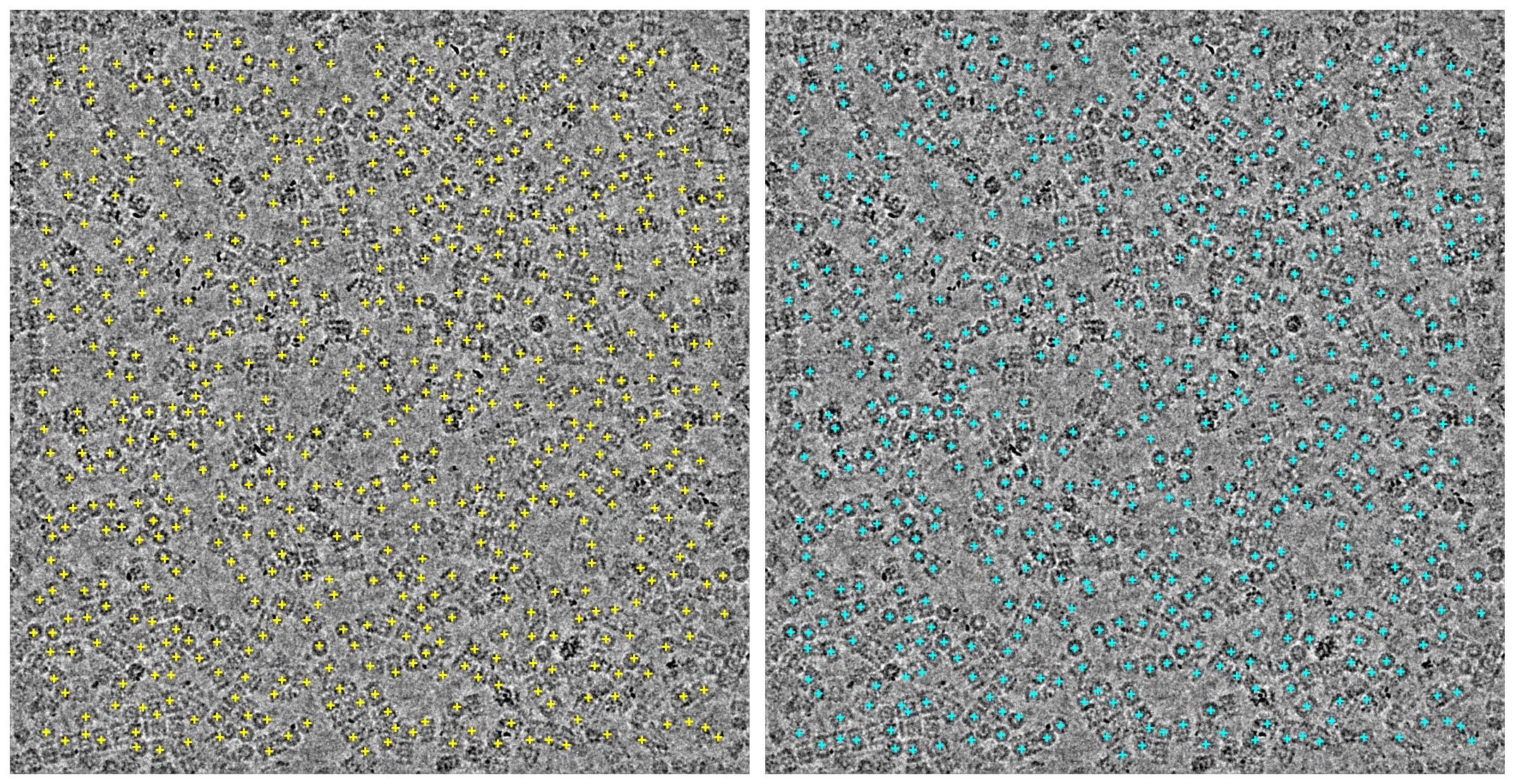
Use matplotlib to render the comparison plots. The following information is required for plotting:

• Downsampled and low-pass filtered micrograph with CryoSPARC’s included utilities

• New downsampled width and height

• The min and maximum color range values, calculated as the 1st and 99th percentile pixel values to eliminate outliers

• The computed (x, y) pixel values at which to plot this micrograph’s particles for the old and new locations

The old and new locations are rendered in yellow and cyan, respectively.

%matplotlib inline

from cryosparc.tools import downsample, lowpass2
import matplotlib.pyplot as plt
import numpy as np

# Initialize a 2x1 plot with axis labels dsiabled
fig, (ax1, ax2) = plt.subplots(ncols=2, figsize=(15, 8), dpi=144)
ax1.axis("off")
ax2.axis("off")

# Downsample and lowpass micrograph
binned = downsample(mic, factor=3)
lowpassed = lowpass2(binned, psize_A=micrograph_psize[0], cutoff_resolution_A=20, order=0.7)
height, width = lowpassed.shape
vmin = np.percentile(lowpassed, 1)
vmax = np.percentile(lowpassed, 99)
ax1.imshow(lowpassed, cmap="gray", vmin=vmin, vmax=vmax, origin="lower")
ax2.imshow(lowpassed, cmap="gray", vmin=vmin, vmax=vmax, origin="lower")

# Plot old particles in yellow
mic_old_particles = particles.query({"location/micrograph_path": mic_path})
old_location_x = mic_old_particles["location/center_x_frac"] * width
old_location_y = mic_old_particles["location/center_y_frac"] * height
ax1.scatter(old_location_x, old_location_y, c="yellow", marker="+")

# Plot new particles in cyan
mic_new_particles = updated_particles.query({"location/micrograph_path": mic_path})
new_location_x = mic_new_particles["location/center_x_frac"] * width
new_location_y = mic_new_particles["location/center_y_frac"] * height
ax2.scatter(new_location_x, new_location_y, c="cyan", marker="+")

fig.tight_layout()

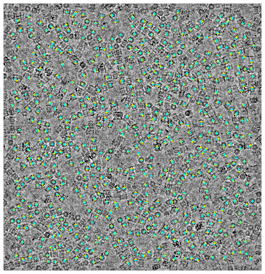
Those same locations overlaid on top of each other

fig = plt.figure(figsize=(7.5, 8), dpi=144)
plt.axis("off")
plt.imshow(lowpassed, cmap="gray", vmin=vmin, vmax=vmax, origin="lower")
plt.scatter(old_location_x, old_location_y, c="yellow", marker="+")
plt.scatter(new_location_x, new_location_y, c="cyan", marker="+")

fig.tight_layout()

Use the project.save_external_result() method with the specified arguments to save the results back to CryoSPARC for extraction and further analysis. The result will be a new “External job” in CryoSPARC in the same workspace as the original job.

Use the slots argument to indicate that only the location/ and alignments2D/ fields have changed.

Specify the passthrough argument as a tuple of the original Select 2D job UID and the output where the particles were loaded from. This ensures that the result is correctly placed in the job tree.

project.save_external_result(
    workspace_uid="W2",
    dataset=updated_particles,
    type="particle",
    name="recentered_particles",
    slots=["location", "alignments2D"],
    passthrough=(job.uid, "particles_selected"),
    title="Recentered particles",
)

'J17'

Look for the “External” job with the number above in the CryoSPARC interface.