3D Flex: Custom Latent Trajectory

3. 3D Flex: Custom Latent Trajectory#

Note

Read the tutorial to learn more about 3D Flexible Refinement.

This example covers the following:

Load particle latent coordinates from a 3D Flex Training job
Plot the latent coordinates
Interactively draw a trajectory through the latent space
Output the trajectory as a new output in CryoSPARC

The resulting trajectory may be used as input to the 3D Flex Generator job to generate a volume series along the trajectory. In this way, you can visualize specific regions or pathways through the latent conformational distribution of the particle.

import json
from pathlib import Path

import numpy as n

from cryosparc.tools import CryoSPARC

with open(Path("~", "instance-info.json").expanduser(), "r") as f:
    credentials = json.load(f)

cs = CryoSPARC(**credentials)
assert cs.test_connection()

Connection succeeded to CryoSPARC command_core at http://cryoem0.sbi:40002
Connection succeeded to CryoSPARC command_vis at http://cryoem0.sbi:40003
Connection succeeded to CryoSPARC command_rtp at http://cryoem0.sbi:40005

Load the particles dataset from the 3D Flex Training job.

import pandas as pd

project = cs.find_project("P312")
particles = project.find_job("J243").load_output("particles")

# only display the first ten rows, since creating an entire dataframe is slow
pd.DataFrame(particles.rows()[:10])

	alignments2D/alpha	alignments2D/alpha_min	alignments2D/class	alignments2D/class_ess	alignments2D/class_posterior	alignments2D/cross_cor	alignments2D/error	alignments2D/image_pow	alignments2D/pose	...	pick_stats/power	pick_stats/template_idx	sym_expand/idx	sym_expand/src_uid	sym_expand/symmetry	uid
0	1.0	1.067518	8	1.000261	0.999869	76.271484	9163.180664	9203.728516	4.744446	...	781.205933	3	0	6947839038024507105	C2	6947839038024507105
1	1.0	1.067518	8	1.000261	0.999869	76.271484	9163.180664	9203.728516	4.744446	...	781.205933	3	1	6947839038024507105	C2	13932325671802011693
2	1.0	0.868515	2	1.006742	0.996642	62.421875	8964.066406	8990.552734	3.205707	...	596.804443	3	0	18174470766076440683	C2	18174470766076440683
3	1.0	0.868515	2	1.006742	0.996642	62.421875	8964.066406	8990.552734	3.205707	...	596.804443	3	1	18174470766076440683	C2	16990665930294442579
4	1.0	1.158005	0	1.656703	0.749064	47.288086	8603.187500	8630.057617	5.385587	...	758.841248	3	0	10868047345897440647	C2	10868047345897440647
5	1.0	1.158005	0	1.656703	0.749064	47.288086	8603.187500	8630.057617	5.385587	...	758.841248	3	1	10868047345897440647	C2	13431911868430011898
6	1.0	0.992612	6	1.032084	0.984298	39.340820	8956.469727	8975.994141	0.000000	...	601.065002	3	0	11087656592019060700	C2	11087656592019060700
7	1.0	0.992612	6	1.032084	0.984298	39.340820	8956.469727	8975.994141	0.000000	...	601.065002	3	1	11087656592019060700	C2	3521966667339501106
8	1.0	0.992270	8	1.000796	0.999602	71.224609	8801.692383	8837.027344	0.128228	...	669.910767	3	0	10759805808414285613	C2	10759805808414285613
9	1.0	0.992270	8	1.000796	0.999602	71.224609	8801.692383	8837.027344	0.128228	...	669.910767	3	1	10759805808414285613	C2	2825550586744122481

10 rows × 110 columns

In this notebook, we create a plot of two of the dimensions and click to generate the trajectory through latent space. This approach necessarily allows only the creation of a trajectory through two of the latent coordinates. If you need to change three or more coordinates simultaneously, you will have to manually create a list of the coordinates you want to use.

selected_dimensions = [0, 2]

Next we create an interative plot that responds to on-click events.

Once the plot is drawn, click repeatedly on the plot along a trajectory you wish to sample in the latent space. The points along this trajectory will form the output of the notebook and be used in 3D Flex Generator.

Note

Using interactive plots in Jupyter Notebooks can present some challenges. Connecting to a remote VS Code remote notebook requires the ipympl package and the %matplotlib widget “magic” line. See the matplotlib documentation for more detail.

%matplotlib widget
from matplotlib import pyplot as plt

fig = plt.figure(figsize=(5, 5))


def do_plot():
    plt.plot(
        particles[f"components_mode_{selected_dimensions[0]}/value"][::10],
        particles[f"components_mode_{selected_dimensions[1]}/value"][::10],
        ".",
        alpha=0.5,
        color="gray",
    )
    plt.grid()


do_plot()
pts = []


def onclick(event):
    fig.clf()
    do_plot()
    pts.append([event.xdata, event.ydata])
    apts = n.array(pts)
    plt.plot(apts[0, 0], apts[0, 1], "xk")
    plt.plot(apts[:, 0], apts[:, 1], ".-r")


cid = plt.gcf().canvas.mpl_connect("button_press_event", onclick)

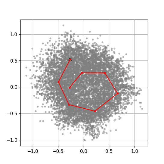
Print out the selected trajectory points. Each column corresponds to the position along that selected coordinate, i.e., in this example column 1 is coordinate 0 and column 2 is coordinate 2.

latent_pts = n.array(pts)
for pt in latent_pts:
    print(f"{pt[0]:5.2f}, {pt[1]:5.2f}")

-0.35,  0.67
-0.78,  0.09
-0.50, -0.67
 0.77, -0.86
 1.06, -0.18
 0.95,  0.56
 0.04,  0.43
-0.27, -0.11

Set up an external job to save the custom latent components. Connect to the train job to ensure output fields get passed through.

# each component has a components_mode_n/component and components_mode_n/value field,
# so we need to divide the components_mode fields by two to get the total number of components
num_components = int(len([x for x in particles.fields() if "components_mode" in x]) / 2)

slot_spec = [{"dtype": "components", "prefix": f"components_mode_{k}", "required": True} for k in range(num_components)]
job = project.create_external_job("W5", "Custom Latents")
job.connect("particles", "J243", "particles", slots=slot_spec)

True

Add and allocate an output for the job to store the custom latent components.

latents_dset = job.add_output(
    type="particle",
    name="latents",
    slots=slot_spec,
    title="Latents",
    alloc=len(latent_pts),
)

Save the points into the allocated dataset.

for k in range(num_components):
    latents_dset[f"components_mode_{k}/component"] = k
    try:
        latents_dset[f"components_mode_{k}/value"] = latent_pts[:, selected_dimensions.index(k)]
    except ValueError:
        # if a coordinate is not in our selected_dimensions, set the trajectory to zero in that coordinate
        latents_dset[f"components_mode_{k}/value"] = 0

Save the output.

with job.run():
    job.save_output("latents", latents_dset)